Identifying Fraud from Enron Emails
Objective
Using the Enron email corpus data to extract and engineer model features, we will attempt to develop a classifier able to identify a "Person of Interest" (PoI) that may have been involved or had an impact on the fraud that occured within the Enron scandal. A list of known PoI has been hand generated from this USATODAY article by the friendly folks at Udacity, who define a PoI as individuals who were indicted, reached a settlement or plea deal with the government, or testified in exchange for prosecution immunity. We will use these PoI labels with the Enron email corpus data to develop the classifier.
Data Structure
The dataset used in this analysis was generated by Udacity and is a dictionary with each person's name in the dataset being the key to each data dictionary. The data dictionaries have the following features:
financial features-=: 'salary', 'deferral_payments', 'total_payments', 'loan_advances', 'bonus', 'restricted_stock_deferred', 'deferred_income', 'total_stock_value', 'expenses', 'exercised_stock_options', 'other', 'long_term_incentive', 'restricted_stock', 'director_fees' - all units are in US dollars
email features: 'to_messages', 'email_address', 'from_poi_to_this_person', 'from_messages', 'from_this_person_to_poi', 'poi', 'shared_receipt_with_poi' -units are generally number of emails messages; notable exception is ‘email_address’, which is a text string
POI label: ‘poi’ -boolean, represented as integer
Model Development Plan
Developing the classification model will consist of 6 steps that can be iterated over until an acceptable model performance is obtained. These steps include: 1. Exploratory Data Analysis on the dataset to understand the data and investigate informative features 2. Select features likely to provide predictive power in the classification model 3. Clean or remove erroneous and outlier data from the selected features 4. Engineer/transform selected features into new features appropriate for classification modelling 5. Test different classifiers and review performance 6. Investigate new data sources that may exist to provide better model performance
Data Exploration and Cleaning
Data Overview
The dataset includes 146 unique individials having 21 features extracted from the email corpus. The amount of feature data for each individual varies. Table 1 summarizes the data count for each feature in the dataset and the count of PoI included in non-nan feature values.
| Feature | Data Count | Count PoI |
|---|---|---|
| name | 146 | 18 |
| poi | 146 | 18 |
| total_stock_value | 126 | 18 |
| total_payments | 125 | 18 |
| email_address | 111 | 18 |
| restricted_stock | 110 | 17 |
| exercised_stock_options | 102 | 12 |
| salary | 95 | 17 |
| expenses | 95 | 18 |
| other | 93 | 18 |
| to_messages | 86 | 14 |
| shared_receipt_with_poi | 86 | 14 |
| from_messages | 86 | 14 |
| from_this_person_to_poi | 86 | 14 |
| from_poi_to_this_person | 86 | 14 |
| bonus | 82 | 16 |
| long_term_incentive | 66 | 12 |
| deferred_income | 49 | 11 |
| deferral_payments | 39 | 5 |
| restricted_stock_deferred | 18 | 0 |
| director_fees | 17 | 0 |
| loan_advances | 4 | 1 |
There are some features in the dataset that having missing information that will be important to our usecase. Some of the features in the dataset will not be very useful in the classification model, as they do not have labelled PoI in their subset of availible data, such as restricted_stock_deferred and director_fees. loan_advances is such a small data sample that it will likely not provide statistically signifigant predictive strength. deferral_payments is borderline, but there are other feature datasets that will likely provide better predictive information. Reviewing the data for missing values, we will exclude restricted_stock_deferred, director_fees, loan_advances and deferral_payments as features from the model.
Outliers
In analyzing the histograms for each feature, a large outlier was noticed across many variables. After further investigation, this turned out to be attributed to an aggreate row of the dataset labelled "TOTAL". This was removed from the dataset.
It also appears that 'LAY KENNETH L' is a large outlier in many features. Kenneth is a PoI however, so we will keep his data for building the classifier and see if we can maintain the ability to build a generalized classifier for the other PoI, as well as for Kenneth.
Data Imputation
In reviewing the dataset, many of the email feature datasets only contain 14 of the 18 identified PoI, while most of the financial features have the full 18 or 17 PoI included. Throwing out data for 20% of our identified PoI seems unnacceptable for such a scarce dataset. Imputing the mean value for any missing email feature seems appropriate, as there is likely a reasonable average number of emails any one employee might send. We will also impute 0 for any financial feature, making the assumption that if the value is missing the employee did not recieve that form of financial compensation. A review of this data imputation may be required as the model is developed and in analyzing the results.
Feature Selection and Engineering
Selection
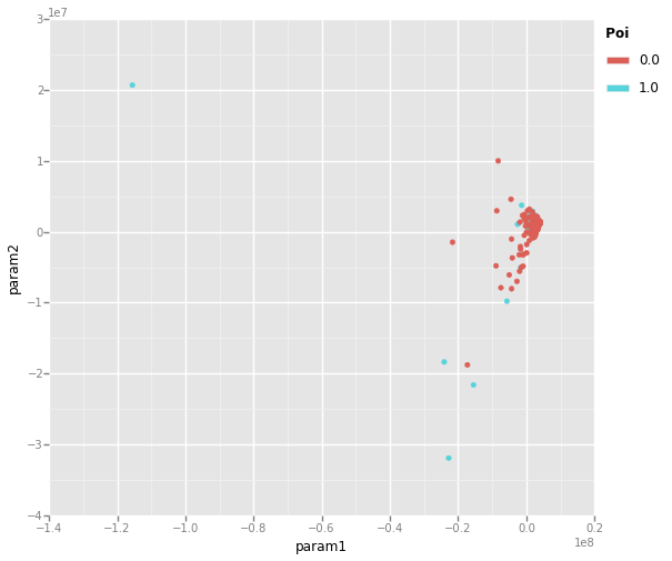
As was discussed above, restricted_stock_deferred, director_fees, loan_advances and deferral_payments have been ommitted as features for the classification model due to their small sample size. There also exists features that are labels instead of useful datum, such as name and email_address. These will not be used as features in the classification model. This leaves us with 15 potentially useful features to select from. Reviewing the data structure, there are two general categories of data: Finanical and Meta-Email. These overarching data categories seem well suited for Primary Component Analysis, to build a featureset that encompasses the most predictive information from the features and avoids dependant features such as total_payments and salary causing erroneous classification or overfitting. Applying PCA to the 15 features to reduce the dimensioanilty to 2 overarching categories, we can visualize the transformed feature relationships.
%matplotlib inline
import numpy as np
import pandas as pd
import pickle
from ggplot import *
from feature_format import featureFormat, targetFeatureSplit
with open("my_dataset.pkl", "r") as data_file:
my_dataset = pickle.load(data_file)
with open("my_feature_list.pkl", "r") as data_file:
features_list = pickle.load(data_file)
data = featureFormat(my_dataset, features_list, sort_keys = True)
labels, features = targetFeatureSplit(data)
#Apply PCA to dataset to allow for visualization
from sklearn.decomposition import PCA
reduced_data = PCA(n_components=2).fit_transform(features)
labels = np.array(labels).reshape(len(reduced_data[:,0]),1)
reduced_data = np.hstack((reduced_data,labels))
df = pd.DataFrame(reduced_data,columns = ['param1', 'param2','poi'])
pca_plt = ggplot(df, aes(x='param1', y='param2', color='poi')) +\
geom_point()
print pca_plt
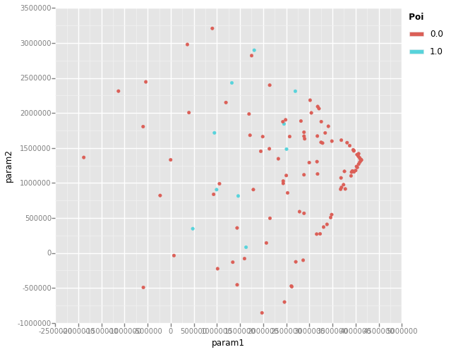
pca_plt_zoomed = pca_plt + xlim(-2500000,5000000) +ylim(-1000000,3500000)
print pca_plt_zoomed
<ggplot: (32479948)>
<ggplot: (32864214)>
Reviewing the PCA plots, there appears to be a few PoI outliers that should be easy to classify, but zooming in on the cluster of datapoints shows PoI data points are very commingled with non-PoI data points that may be difficult to adequately classify. This model may need more advanced features to develop an adequate classifier.
Feature Engineering
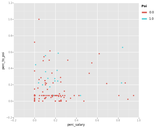
It is likely that additional features are required to adequately model a PoI classifier. Most of the supplied features are absolute values of a persons' financial compensation or email correspondance. It makes sense that a more relative measure of these features is appropriate to use when comparing whether someone is a PoI or not. Three additional features have been engineered for use in classifier development:
1. perc_salary - The percentage each employees' salary makes of of their total payment, defined as salary/total_payments. This will represent if the employees compensation is made up of complex additional payments or just a basic salary.
2. perc_to_poi - The percentage of employees total sent emails to a PoI. This will represent the degree an employee spends their time interacting with a PoI.
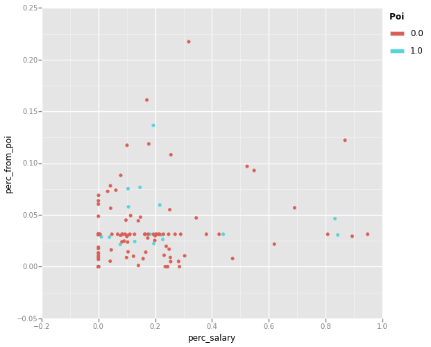
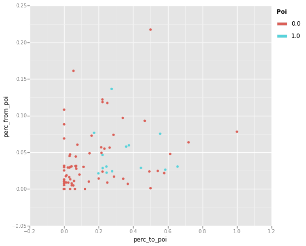
3. perc_from_poi - The percentage of employees total recieved emails from a PoI. This will represent the degree a PoI spends their time interacting with an employee.
eng_data = np.hstack((data[:,(16,17,18)],labels))
df = pd.DataFrame(eng_data,columns = ['perc_salary', 'perc_to_poi','perc_from_poi','poi'])
print ggplot(df, aes(x='perc_salary', y='perc_to_poi', color='poi')) +\
    geom_point()
print ggplot(df, aes(x='perc_salary', y='perc_from_poi', color='poi')) +\
    geom_point()
print ggplot(df, aes(x='perc_to_poi', y='perc_from_poi', color='poi')) +\
geom_point()
<ggplot: (36868016)>
<ggplot: (35575721)>
<ggplot: (36864902)>
In reviewing the plots, both the perc_to_poi vs perc_salary and the perc_from_poi vs perc_to_poi plots show good seperation of PoI from non-PoI datapoints. The perc_from_poi vs perc_salary plot shows less of a seperation, with many PoI data points closely clustered with non-PoI datum. These advanced features seem to show more promise then the simple PCA approach above, but we will test and compare the relative performance of tuned classifiers using the two approaches.
Model Development, Tuning and Evaluation
Using sklearn's Machine Learning Map as a guide, we will test the PCA and advanced feature datasets with various classifier algorithms and tuning parameters in an attempt to develop the optimal PoI classifier. Sklearn's pipeline and gridsearch modules will be helpful in performing this analysis. We will also use sklearns StandardScaler to scale out input datasets, as some of our classifier algorithms highly recommend the use of scalled variables, like the svm classifer which is not scale invariant.
Model Validation
In order to determine which model has the "best" performance, model validation is required to prove the models ability to make correct predictions on a generalized dataset. Model validation is the method of extracting a subset of a dataset, known as the test data, training a model excluding this extraction and feeding the model with the extracted dataset to test its performance in predicting the known results of the extracted dataset. This is important to allow for the quantified comparasion of different models.
To compare the performance of each tuned model, we will use Udacity's test_classifier function. This function uses Precision and Recall as the performance metrics for each model. The Precision of the classifier is its ability to correctly identify PoI without incorrectly labelling people that are not PoI as a PoI. The Recall of the classifier is its ability to correctly identify all of the PoI that should be identified. In order to perform the validation classification, the test function uses sklearns StratifiedShuffleSplit method to split the dataset into training and test data. This allows us to maximize the data points used in both the training and testing datasets by performing multiple training and validation experiments on a shuffled subset of the full dataset. Being a fairly sparse dataset with only 18 labelled examples of PoIs, it is important for the testing methodology to perform on multiple interations of training and test data to ensure accurate performance results. It is also important to include shuffling in the test data selection to ensure a random distribution of PoI and non-PoI data points in each dataset.
PCA Featureset Model
from sklearn.pipeline import Pipeline
from sklearn import svm
from sklearn.grid_search import GridSearchCV
from sklearn.neighbors import KNeighborsClassifier
from sklearn.ensemble import RandomForestClassifier
from sklearn.preprocessing import StandardScaler
from sklearn.cross_validation import train_test_split
from sklearn.decomposition import PCA
import tester


data = featureFormat(my_dataset, features_list, sort_keys = True)
labels, features = targetFeatureSplit(data)

pca_svm = Pipeline([('pca',PCA(n_components=2)),('scaler',StandardScaler()),('svm',svm.SVC())])
param_grid = ([{'svm__C': [1000,10000],
                'svm__gamma': [0.01,0.0001],
                'svm__degree':[2,3],
                'svm__kernel': ['linear','rbf','poly']}])
svm_clf = GridSearchCV(pca_svm,param_grid,scoring='recall').fit(features,labels).best_estimator_
pca_knb = Pipeline([('pca',PCA(n_components=2)),('scaler',StandardScaler()),('knb',KNeighborsClassifier())])
param_grid = ([{'knb__n_neighbors': [4,5,6]}])
knb_clf = GridSearchCV(pca_knb,param_grid,scoring='recall').fit(features,labels).best_estimator_
pca_rfst = Pipeline([('pca',PCA(n_components=2)),('scaler',StandardScaler()),
                 ('rfst',RandomForestClassifier())])
param_grid = ([{'rfst__n_estimators': [4,5,6]}])
rfst_clf = GridSearchCV(pca_rfst,param_grid,scoring='recall').fit(features,labels).best_estimator_

print svm_clf
tester.test_classifier(svm_clf,my_dataset,features_list)
print knb_clf
tester.test_classifier(knb_clf,my_dataset,features_list)
print rfst_clf
tester.test_classifier(rfst_clf,my_dataset,features_list)
Pipeline(steps=[('pca', PCA(copy=True, n_components=2, whiten=False)), ('scaler', StandardScaler(copy=True, with_mean=True, with_std=True)), ('svm', SVC(C=1000, cache_size=200, class_weight=None, coef0=0.0, degree=2,
  gamma=0.01, kernel='rbf', max_iter=-1, probability=False,
  random_state=None, shrinking=True, tol=0.001, verbose=False))])
    Accuracy: 0.87573   Precision: 0.68579  Recall: 0.12550 F1: 0.21217 F2: 0.15001
    Total predictions: 15000    True positives:  251    False positives:  115   False negatives: 1749   True negatives: 12885

Pipeline(steps=[('pca', PCA(copy=True, n_components=2, whiten=False)), ('scaler', StandardScaler(copy=True, with_mean=True, with_std=True)), ('knb', KNeighborsClassifier(algorithm='auto', leaf_size=30, metric='minkowski',
           metric_params=None, n_neighbors=4, p=2, weights='uniform'))])
    Accuracy: 0.86807   Precision: 0.54393  Recall: 0.06500 F1: 0.11612 F2: 0.07889
    Total predictions: 15000    True positives:  130    False positives:  109   False negatives: 1870   True negatives: 12891

Pipeline(steps=[('pca', PCA(copy=True, n_components=2, whiten=False)), ('scaler', StandardScaler(copy=True, with_mean=True, with_std=True)), ('rfst', RandomForestClassifier(bootstrap=True, class_weight=None, criterion='gini',
            max_depth=None, max_features='auto', max_leaf_nodes=None,
            min_samples_leaf=1, min_samples_split=2,
            min_weight_fraction_leaf=0.0, n_estimators=6, n_jobs=1,
            oob_score=False, random_state=None, verbose=0,
            warm_start=False))])
    Accuracy: 0.83913   Precision: 0.25150  Recall: 0.10450 F1: 0.14765 F2: 0.11833
    Total predictions: 15000    True positives:  209    False positives:  622   False negatives: 1791   True negatives: 12378
Reviewing the results, we see that the svm and KNeighbors classifiers have fairly good Precision, meaning they are able to properly identify PoI wihout too many incorrectly labelled PoI. The RandomForestClassiefier has poorer Precision performance. The Recall for all classifiers is rather poor, with the svm classifier having the highest Recall at 0.1255. This indicates that, although the classifiers do not miss-label many non-PoI employees, they tend to under-label correctly people that should be considered PoI. Considering the use case for this model is likely to be a filter that could provide a short-list of people to investigate further, having a high Recall is important to ensure the short-list captures people that are likely to be PoI. Given this, it is likely the above classifiers are not performant enough to provide sufficient value in this investigation. From visual inspection it was seen that the data relationships showed little classifcation potential and after exhaustively tuning these classifiers, that interpretation seems to be correct. The PCA featureset does not seem to provide enough informative characteristics to build a suitable classifier, and further feature engineering is likely required.
Engineered Feature Model
from sklearn.feature_selection import SelectKBest

eng_svm = Pipeline([('scaler',StandardScaler()),('kbest',SelectKBest()),('svm',svm.SVC())])
param_grid = ([{'kbest__k':[3,4,5,6],
                'svm__C': [1,10,100,1000],
                'svm__gamma': [1,0.1,0.01,0.001],
                'svm__degree':[2,3,4],
                'svm__kernel': ['linear','rbf','poly']}])
svm_clf = GridSearchCV(eng_svm,param_grid,scoring='recall').fit(features,labels).best_estimator_
eng_knb = Pipeline([('scaler',StandardScaler()),('kbest',SelectKBest()),('knb',KNeighborsClassifier())])
param_grid = ([{'kbest__k':[3,4,5,6],'knb__n_neighbors': [2,3,4,5,6]}])
knb_clf = GridSearchCV(eng_knb,param_grid,scoring='recall').fit(features,labels).best_estimator_
eng_rfst = Pipeline([('scaler',StandardScaler()),('kbest',SelectKBest()),
                 ('rfst',RandomForestClassifier())])
param_grid = ([{'kbest__k':[3,4,5,6],'rfst__n_estimators': [2,3,4,5,6]}])
rfst_clf = GridSearchCV(eng_rfst,param_grid,scoring='recall').fit(features,labels).best_estimator_

print svm_clf
tester.test_classifier(svm_clf,my_dataset,features_list)
print knb_clf
tester.test_classifier(knb_clf,my_dataset,features_list)
print rfst_clf
tester.test_classifier(rfst_clf,my_dataset,features_list)
Pipeline(steps=[('scaler', StandardScaler(copy=True, with_mean=True, with_std=True)), ('kbest', SelectKBest(k=6, score_func=<function f_classif at 0x000000001F36F128>)), ('svm', SVC(C=1, cache_size=200, class_weight=None, coef0=0.0, degree=4, gamma=1,
  kernel='poly', max_iter=-1, probability=False, random_state=None,
  shrinking=True, tol=0.001, verbose=False))])
    Accuracy: 0.81753   Precision: 0.25351  Recall: 0.18950 F1: 0.21688 F2: 0.19958
    Total predictions: 15000    True positives:  379    False positives: 1116   False negatives: 1621   True negatives: 11884

Pipeline(steps=[('scaler', StandardScaler(copy=True, with_mean=True, with_std=True)), ('kbest', SelectKBest(k=3, score_func=<function f_classif at 0x000000001F36F128>)), ('knb', KNeighborsClassifier(algorithm='auto', leaf_size=30, metric='minkowski',
           metric_params=None, n_neighbors=3, p=2, weights='uniform'))])
    Accuracy: 0.86127   Precision: 0.46341  Recall: 0.25650 F1: 0.33022 F2: 0.28165
    Total predictions: 15000    True positives:  513    False positives:  594   False negatives: 1487   True negatives: 12406

Pipeline(steps=[('scaler', StandardScaler(copy=True, with_mean=True, with_std=True)), ('kbest', SelectKBest(k=4, score_func=<function f_classif at 0x000000001F36F128>)), ('rfst', RandomForestClassifier(bootstrap=True, class_weight=None, criterion='gini',
            max_depth=None, max_features='auto', max_l...n_jobs=1,
            oob_score=False, random_state=None, verbose=0,
            warm_start=False))])
    Accuracy: 0.83020   Precision: 0.32066  Recall: 0.24450 F1: 0.27745 F2: 0.25669
    Total predictions: 15000    True positives:  489    False positives: 1036   False negatives: 1511   True negatives: 11964
Although we managed to improve our best Recall score with a tuned KNeibors Classifier, the Precision performance was dramitacally reduced. At this point, it would likely be beneficial to perform anothet iteration of the model development process in order to better explore the data, develop features and investigate other classisifier algorithms. However, there is one more approach that may be useful to investigate: developing a hybrid model by combining the two input theories outlined above.
Hybrid Model
Using sklearns FeatureUninion module, we can combine the PCA reduced dimensionality dataset with the engineered feature dataset as a hybrid featureset for model development.
from sklearn.pipeline import FeatureUnion

combined_features = FeatureUnion([("pca", PCA()), ("kbest", SelectKBest())])

hybrid_svm = Pipeline([('features',combined_features),('scaler',StandardScaler()),('svm',svm.SVC())])
param_grid = ([{'features__pca__n_components':[2,3,4,5,6,7],'features__kbest__k':[2,3,4,5,6,7],
                'svm__C': [1,10,100,1000],
                'svm__gamma': [1,0.1,0.01,0.001],
                'svm__degree':[2,3,4],
                'svm__kernel': ['rbf','poly']}])
svm_clf = GridSearchCV(hybrid_svm,param_grid,scoring='recall').fit(features,labels).best_estimator_
hybrid_knb = Pipeline([('features',combined_features),('scaler',StandardScaler()),('knb',KNeighborsClassifier())])
param_grid = ([{'features__pca__n_components':[2,3,4,5,6],'features__kbest__k':[2,3,4,5,6],'knb__n_neighbors': [1,2,3,4,5,6,7]}])
knb_clf = GridSearchCV(hybrid_knb,param_grid,scoring='recall').fit(features,labels).best_estimator_
hybrid_rfst = Pipeline([('features',combined_features),('scaler',StandardScaler()),
                 ('rfst',RandomForestClassifier())])
param_grid = ([{'features__pca__n_components':[2,3,4,5,6],'features__kbest__k':[2,3,4,5,6],'rfst__n_estimators': [2,3,4,5,6,7]}])
rfst_clf = GridSearchCV(hybrid_rfst,param_grid,scoring='recall').fit(features,labels).best_estimator_

print svm_clf
tester.test_classifier(svm_clf,my_dataset,features_list)
print knb_clf
tester.test_classifier(knb_clf,my_dataset,features_list)
print rfst_clf
tester.test_classifier(rfst_clf,my_dataset,features_list)
Pipeline(steps=[('features', FeatureUnion(n_jobs=1,
       transformer_list=[('pca', PCA(copy=True, n_components=7, whiten=False)), ('kbest', SelectKBest(k=5, score_func=<function f_classif at 0x000000001F36F128>))],
       transformer_weights=None)), ('scaler', StandardScaler(copy=True, with_mean=True, with...y', max_iter=-1, probability=False, random_state=None,
  shrinking=True, tol=0.001, verbose=False))])
    Accuracy: 0.82167   Precision: 0.33234  Recall: 0.33450 F1: 0.33342 F2: 0.33407
    Total predictions: 15000    True positives:  669    False positives: 1344   False negatives: 1331   True negatives: 11656

Pipeline(steps=[('features', FeatureUnion(n_jobs=1,
       transformer_list=[('pca', PCA(copy=True, n_components=4, whiten=False)), ('kbest', SelectKBest(k=6, score_func=<function f_classif at 0x000000001F36F128>))],
       transformer_weights=None)), ('scaler', StandardScaler(copy=True, with_mean=True, with_std=True)), ('knb', KNeighborsClassifier(algorithm='auto', leaf_size=30, metric='minkowski',
           metric_params=None, n_neighbors=1, p=2, weights='uniform'))])
    Accuracy: 0.80880   Precision: 0.22462  Recall: 0.17700 F1: 0.19799 F2: 0.18484
    Total predictions: 15000    True positives:  354    False positives: 1222   False negatives: 1646   True negatives: 11778

Pipeline(steps=[('features', FeatureUnion(n_jobs=1,
       transformer_list=[('pca', PCA(copy=True, n_components=2, whiten=False)), ('kbest', SelectKBest(k=5, score_func=<function f_classif at 0x000000001F36F128>))],
       transformer_weights=None)), ('scaler', StandardScaler(copy=True, with_mean=True, with...n_jobs=1,
            oob_score=False, random_state=None, verbose=0,
            warm_start=False))])
    Accuracy: 0.83400   Precision: 0.32771  Recall: 0.23300 F1: 0.27236 F2: 0.24729
    Total predictions: 15000    True positives:  466    False positives:  956   False negatives: 1534   True negatives: 12044
The Hybrid model was able to develop a classifier that satisfies the minimun target of 0.3 for both Precision and Recall with an SVM classifier. Although the model's Precision is reduced compared to previous iterations, it is better suited for correctly identifier employees that are PoI in order to develop a short-list of people to investigate further.
Final Model
import operator
combined_features = FeatureUnion([("pca", PCA(n_components=7)), ("kbest", SelectKBest(k=6))])
final_svm = Pipeline([('features',combined_features),('scaler',StandardScaler()),
                    ('svm',svm.SVC(C=1,degree=3,kernel='poly',gamma=1))])
svm_clf = final_svm.fit(features,labels)
feature_scores = sorted({features_list[i]:svm_clf.get_params()['features'].get_params()['kbest'].scores_[i]
                         for i in range(0,18)}.items(),reverse=True, key=operator.itemgetter(1))
print feature_scores
print svm_clf.get_params()
tester.test_classifier(svm_clf,my_dataset,features_list)
[('restricted_stock', 25.380105299760199), ('from_poi_to_this_person', 24.752523020258508), ('other', 21.327890413979102), ('exercised_stock_options', 18.861795316466416), ('perc_salary', 16.719777335704574), ('long_term_incentive', 11.732698076065354), ('bonus', 10.222904205832778), ('total_payments', 9.4807432034789336), ('total_stock_value', 8.9678193476776205), ('salary', 6.3746144901977475), ('to_messages', 5.7652373136035786), ('expenses', 4.2635766381444693), ('from_this_person_to_poi', 3.0545709279872115), ('deferred_income', 2.8591257010691469), ('perc_to_poi', 1.5752718701560835), ('from_messages', 1.3690711377259386), ('shared_receipt_with_poi', 0.58945562335007018), ('poi', 0.37046177768797534)]
{'features': FeatureUnion(n_jobs=1,
       transformer_list=[('pca', PCA(copy=True, n_components=7, whiten=False)), ('kbest', SelectKBest(k=6, score_func=<function f_classif at 0x000000001F36F128>))],
       transformer_weights=None), 'scaler': StandardScaler(copy=True, with_mean=True, with_std=True), 'features__pca__copy': True, 'svm__shrinking': True, 'svm__gamma': 1, 'svm__verbose': False, 'svm__probability': False, 'features__pca__whiten': False, 'features__kbest__k': 6, 'features__kbest__score_func': <function f_classif at 0x000000001F36F128>, 'svm__cache_size': 200, 'scaler__copy': True, 'svm__degree': 3, 'scaler__with_mean': True, 'features__kbest': SelectKBest(k=6, score_func=<function f_classif at 0x000000001F36F128>), 'svm__kernel': 'poly', 'svm__max_iter': -1, 'svm__coef0': 0.0, 'svm__random_state': None, 'scaler__with_std': True, 'svm': SVC(C=1, cache_size=200, class_weight=None, coef0=0.0, degree=3, gamma=1,
  kernel='poly', max_iter=-1, probability=False, random_state=None,
  shrinking=True, tol=0.001, verbose=False), 'features__pca__n_components': 7, 'svm__C': 1, 'svm__class_weight': None, 'svm__tol': 0.001, 'features__pca': PCA(copy=True, n_components=7, whiten=False)}
    Accuracy: 0.81413   Precision: 0.31398  Recall: 0.33250 F1: 0.32297 F2: 0.32862
    Total predictions: 15000    True positives:  665    False positives: 1453   False negatives: 1335   True negatives: 11547
Conclusions and Reflection
In this analysis, we attempted to build a classification model that could predict whether someone is likely to be a Person of Interest (PoI) in the Enron scandal given their email and financial data. After exploring the data and removing outliers, we investigated two input featuresets: PCA transformed data and engineered features that provided a normalized representation of the email and financial data. Applying multiple classifier algorithms and tuning via GridSearch, the final model was developed which consisted of using a hybrid of the PCA and engineered featureset as the model inputs and a polynomial svm classifier with degree 3 and C and gamme values both 1. This final classifier was selected by reviewing the comparative performance of each models' Precision and Recall scores, with the selected model having a Precision of 0.314 and Recall of 0.333. These performance metrics were chosen as they provide a balance between the goal of producing a short-list of potential PoI candidates to flag for further investigation, while preventing the over classification of non-PoI individuals. Using other performance metrics, such as accuracy in this situation would lead to sub-optimal classifiers, as the number of correct predictions is not as useful as ensuring people that are PoI's are identified as such. This can be a common pitfall of performance measurement, and the goal of the model needs to be well defined before its performance can be measured.
Using the GridSearch functionality of sklearn allowed for the automated tuning of the classifier algorithms. This tuning allowed for the use of different parameters in the classifiers, such as the type of svm (linear, rbf or polynomial) or the number of nearest neighbors to use in the KNeighbors classifier. This tuning is important in producing an effective classifier, as different datasets will result in different patterns. A linear svm may work well with clearly split datasets, but a polynimal svm will be better suited to datasets that result in curved patterns. Without correctly tuning the classification algorithms, a sufficient model will be difficult to develop.
Although the final model meets the minimum goal of Precision and Recall >0.3, there is likely a more optimal classifier that could be developed by further exploring the dataset, engineering more intelligent features and investigating other classifier algorithms better suited to this problem. This model is also likely overfitted to this dataset and probably not directly useful in future investigations, but the proof of concept could be utilized by the investigators to generate their own model as they begin to identify PoI in their own investigation of a similiar nature to the Enron scandal. It would also be interesting to investigate if other features can be developed to help identify potential PoI, such as performing Natural Language Processing on the content of email messages to descern if any conversation patterns emerged between PoI.