MAI-IML Exercise 4: Adaboost from Scratch and Predicting Customer Churn

Abstract

In this work, we develop a custom adaboost classifier compatible with the sklearn package and test it on a dataset from a telecommunication company requiring the correct classification of custumers likely to "churn", or quit their services, for use in developing investment plans to retain these high risk customers.

Adaboost from Scratch

Defined below is an sklearn compatable estimator utilizing the adaboost algorithm to perform binary classification. The input parameters for this estimator is the number of weak learners (which are decision tree stubs on a single, randomly selected feature) to train and aggregate to produce the final classifier. An optional weight distribution can also be passed to the classifier, which defaults to uniform if not set. This custom estimator will later be utilized to develop a classifier capable of predicting customer churn from labelled customer data.

#imports  
%matplotlib inline  
import warnings  
warnings.filterwarnings('ignore')  
import pandas as pd  
import numpy as np  
import matplotlib.pyplot as plt  
from pandas.tools.plotting import scatter_matrix  
import seaborn as sns  
from sklearn.feature_selection import SelectKBest  
from sklearn.pipeline import Pipeline  
from sklearn.model_selection import GridSearchCV  
from sklearn.model_selection import train_test_split  
from sklearn.preprocessing import OneHotEncoder  
from sklearn.metrics import confusion_matrix

#Custom Classifier  
from sklearn.utils.estimator_checks import check_estimator  
from sklearn.base import BaseEstimator, ClassifierMixin  
from sklearn.utils.validation import check_X_y, check_array, check_is_fitted  
from sklearn.utils.multiclass import unique_labels  
class IMLAdaBoostClassifier(BaseEstimator, ClassifierMixin):  

    """ IML implementation of an Adaboost Classifier.
    An implementation of the Adaboost algorithm for classification using decision stubs as the weak learner with n_estimators
    parameter. Weights are initalized as uniform, 1/N and learning rate alpha is calculated using 1/2ln(1-err/err) at each
    estimator timestep.
    Parameters
    ----------
    n_estimators : integer, optional (default=50)
        The maximum number of estimators at which boosting is terminated.
    weights : list, optional (default=uniform)
      The distribution of weights for each example
    Attributes
    ----------
    weak_learners : 3-tuple of weak_learner stub definition of - [feature stub column index, stub split value, greater then or less
    then equality tag]
    classes_ : array of shape = [n_classes]
        The classes labels.
    alphas : array of floats
        Weights for each estimator in the boosted ensemble.
    """

    def __init__(self, n_estimators=50,weights=[]):
        self.n_estimators = n_estimators
        self.weak_learners = []
        self.alphas = []
        self.weights = weights

    def fit(self, X, y):

        # Check that X and y have correct shape
        X, y = check_X_y(X, y)
        # Store the classes seen during fit
        self.classes_ = unique_labels(y)
        #initialize wents with uniform distribution
        if self.weights == []:
            weights = [1/len(y) for lbl in y]
        else:
            weights = self.weights
        for n in range(self.n_estimators):
            #for each n estimator, build and store the weak learner with associated alpha's
            weak_learner, alpha, weights = self.decision_stump(X,y,weights)
            if weak_learner:
                self.weak_learners.append(weak_learner)
                self.alphas.append(alpha)
        self.alphas = [tmp_a/sum(self.alphas) for tmp_a in self.alphas]#normalize final alphas
        self.X_ = X
        self.y_ = y
        # Return the classifier

        return self

    def predict(self, X):

        # Check is fit had been called
        check_is_fitted(self, ['X_', 'y_'])

        # Input validation
        X = check_array(X)

        #for each predicting sample, aggregate the weak_learnings by weighted sum and return the sign of the result as the pred
        df_preds = self.decision_function(X)
        preds = np.array([np.sign(tmp_pred) for tmp_pred in df_preds])
        return preds

    def decision_function(self, X):
        preds = []
        for smpl in X:
            tmp_pred = 0
            for i,estimator in enumerate(self.weak_learners):
                #get feature and split value from 3-tuple weak_learner [split_feature_indx,split_value, 'gt' or 'lt' tag]
                split_feature = estimator[0]
                split_value = estimator[1]
                #check the weak_learner inequality rule for the smpl and increment aggregation function
                if estimator[2] == 'gt':
                    if smpl[split_feature] >= split_value:
                        tmp_pred = tmp_pred + self.alphas[i]*1
                    else:
                        tmp_pred = tmp_pred + self.alphas[i]*-1
                elif estimator[2] == 'lt':
                    if smpl[split_feature] <= split_value:
                        tmp_pred = tmp_pred + self.alphas[i]*1
                    else:
                        tmp_pred = tmp_pred + self.alphas[i]*-1
            preds.append(tmp_pred)
        return np.array(preds)

    def decision_stump(self,X,y,weights):
        #create a weak_learning by creating a decision stump by selecting a random feature to split on, using the values
        #in the feature as split values to test until a weak learner (< 50% error) is found for either the greater then or 
        #less then split value inequality test. return the created weak learning, updated weights and associated alpha
        rnd_column_indx = np.random.randint(0,X.shape[1])
        rnd_column = X[:,rnd_column_indx]
        weak_learner = []
        alpha = 0
        unique_vals = list(set(rnd_column)) #create a shuffled list of unique values in selected column to test split values from
        np.random.shuffle(unique_vals)
        for split_val in unique_vals:
            #check the error rates for stub with split value for < or > rule, if err <50% return resulting weak_learner, alpha
            #and new weights
            gt_prd_labels = [1 if check_val >= split_val else -1 for check_val in rnd_column]
            #add small error amount to prevent div by 0 error
            gt_err = sum([0 if y[i]*gt_prd_labels[i] == 1 else (1*weights[i]) for i in range(len(y))]) + 0.0000001
            lt_prd_labels = [1 if check_val <= split_val else -1 for check_val in rnd_column]
            lt_err = sum([0 if y[i]*lt_prd_labels[i] == 1 else (1*weights[i]) for i in range(len(y))]) + 0.0000001
            if gt_err < 0.5: 
                alpha = 0.5*np.log((1-gt_err)/gt_err)
                weights = [weights[i]*np.exp(-alpha*y[i]*gt_prd_labels[i]) for i in range(len(y))]
                weak_learner = [rnd_column_indx,split_val,'gt']
                return weak_learner, alpha, weights
            elif lt_err < 0.5:
                alpha = 0.5*np.log((1-lt_err)/lt_err)
                weights = [weights[i]*np.exp(-alpha*y[i]*lt_prd_labels[i]) for i in range(len(y))]
                weak_learner = [rnd_column_indx,split_val,'lt']
                return weak_learner, alpha, weights
        print ("No Weak Learner Found for feature " + str(rnd_column_indx))
        return weak_learner,alpha,weights

Estimator Testing

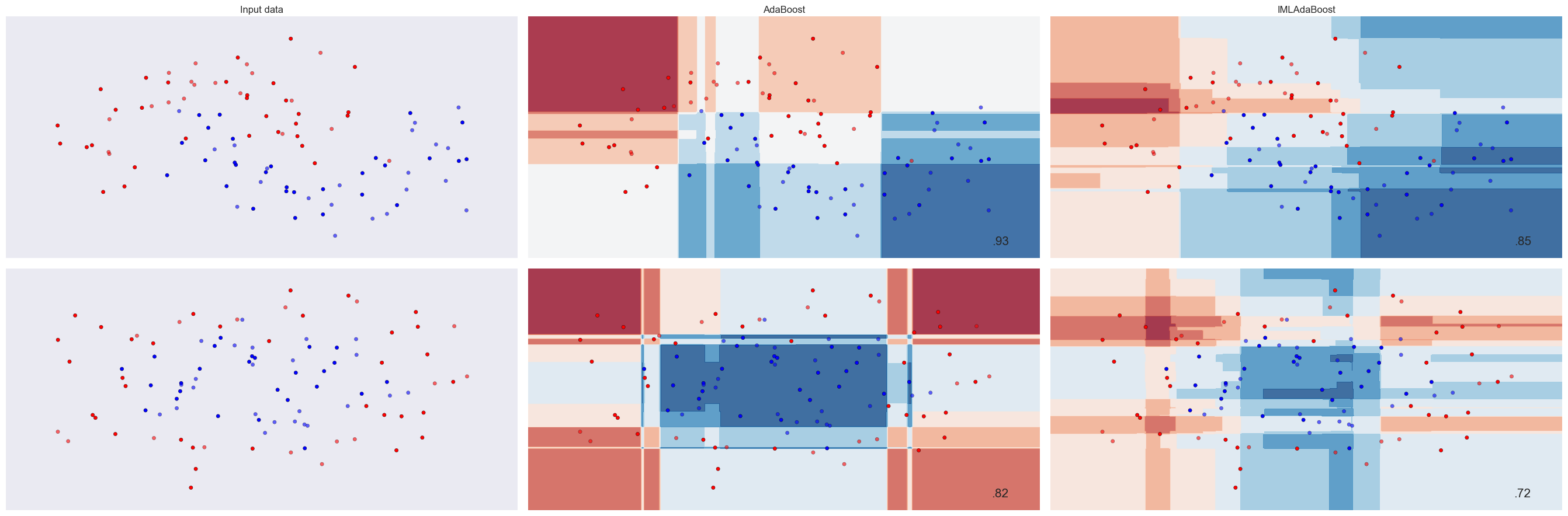
To ensure the estimator has been properly coded, we compare the results on a couple datasets with the packaged adabooster in sklearn. Visualizing the results, we can see the estimator is performing as expected, with similiar results as the sklearn adabooster. The differences likely stem from our custom estimator not encorporating any intelligence in the decision stubs, simply naively selecting any that perform better than random as the weak learning, where sklearns adaboost utilizes decisiontree classifiers as their stubs which optimize the stub splitting based on information gain metrics.

# Code source: Gaël Varoquaux
#              Andreas Müller
# Modified for documentation by Jaques Grobler
# License: BSD 3 clause

from matplotlib.colors import ListedColormap
from sklearn.model_selection import train_test_split
from sklearn.preprocessing import StandardScaler
from sklearn.datasets import make_moons, make_circles, make_classification
from sklearn.ensemble import RandomForestClassifier, AdaBoostClassifier

h = .02  # step size in the mesh

names = ["AdaBoost","IMLAdaBoost"]

classifiers = [
    AdaBoostClassifier(),
    IMLAdaBoostClassifier(n_estimators=25)

]


X, y = make_classification(n_features=2, n_redundant=0, n_informative=2,
                           random_state=1, n_clusters_per_class=1)
y = [-1 if tmp_y == 0 else 1 for tmp_y in y]
rng = np.random.RandomState(2)
X += 2 * rng.uniform(size=X.shape)

datasets = [make_moons(noise=0.3, random_state=0),
            make_circles(noise=0.2, factor=0.5, random_state=1),
            ]

figure = plt.figure(figsize=(27, 9))
i = 1
# iterate over datasets
for ds_cnt, ds in enumerate(datasets):
    # preprocess dataset, split into training and test part
    X, y = ds
    y = [-1 if tmp_y == 0 else 1 for tmp_y in y]
    X = StandardScaler().fit_transform(X)
    X_train, X_test, y_train, y_test = \
        train_test_split(X, y, test_size=.4, random_state=42)

    x_min, x_max = X[:, 0].min() - .5, X[:, 0].max() + .5
    y_min, y_max = X[:, 1].min() - .5, X[:, 1].max() + .5
    xx, yy = np.meshgrid(np.arange(x_min, x_max, h),
                         np.arange(y_min, y_max, h))

    # just plot the dataset first
    cm = plt.cm.RdBu
    cm_bright = ListedColormap(['#FF0000', '#0000FF'])
    ax = plt.subplot(len(datasets), len(classifiers) + 1, i)
    if ds_cnt == 0:
        ax.set_title("Input data")
    # Plot the training points
    ax.scatter(X_train[:, 0], X_train[:, 1], c=y_train, cmap=cm_bright)
    # and testing points
    ax.scatter(X_test[:, 0], X_test[:, 1], c=y_test, cmap=cm_bright, alpha=0.6)
    ax.set_xlim(xx.min(), xx.max())
    ax.set_ylim(yy.min(), yy.max())
    ax.set_xticks(())
    ax.set_yticks(())
    i += 1

    # iterate over classifiers
    for name, clf in zip(names, classifiers):
        ax = plt.subplot(len(datasets), len(classifiers) + 1, i)
        clf.fit(X_train, y_train)
        score = clf.score(X_test,y_test)

        # Plot the decision boundary. For that, we will assign a color to each
        # point in the mesh [x_min, x_max]x[y_min, y_max].
        if hasattr(clf, "decision_function"):
            Z = clf.decision_function(np.c_[xx.ravel(), yy.ravel()])
        else:
            Z = clf.predict_proba(np.c_[xx.ravel(), yy.ravel()])[:, 1]

        # Put the result into a color plot
        Z = Z.reshape(xx.shape)
        ax.contourf(xx, yy, Z, cmap=cm, alpha=.8)

        # Plot also the training points
        ax.scatter(X_train[:, 0], X_train[:, 1], c=y_train, cmap=cm_bright)
        # and testing points
        ax.scatter(X_test[:, 0], X_test[:, 1], c=y_test, cmap=cm_bright,
                   alpha=0.6)

        ax.set_xlim(xx.min(), xx.max())
        ax.set_ylim(yy.min(), yy.max())
        ax.set_xticks(())
        ax.set_yticks(())
        if ds_cnt == 0:
            ax.set_title(name)
        ax.text(xx.max() - .3, yy.min() + .3, ('%.2f' % score).lstrip('0'),
                size=15, horizontalalignment='right')
        i += 1

plt.tight_layout()
plt.show()

Customer Churn Exploratory Data Analysis

Below is a preliminary Exploratory Data Analysis of the customer churn data to help discover any data inconsistencies and provide an intuition for developing a model of customer churn.

df = pd.read_csv("churn.csv")
df.head()

	State	Account Length	Area Code	Phone	Int'l Plan	VMail Plan	VMail Message	Day Mins	Day Calls	Day Charge	...	Eve Calls	Eve Charge	Night Mins	Night Calls	Night Charge	Intl Mins	Intl Calls	Intl Charge	CustServ Calls	Churn?
0	KS	128	415	382-4657	no	yes	25	265.1	110	45.07	...	99	16.78	244.7	91	11.01	10.0	3	2.70	1	False
1	OH	107	415	371-7191	no	yes	26	161.6	123	27.47	...	103	16.62	254.4	103	11.45	13.7	3	3.70	1	False
2	NJ	137	415	358-1921	no	no	0	243.4	114	41.38	...	110	10.30	162.6	104	7.32	12.2	5	3.29	0	False
3	OH	84	408	375-9999	yes	no	0	299.4	71	50.90	...	88	5.26	196.9	89	8.86	6.6	7	1.78	2	False
4	OK	75	415	330-6626	yes	no	0	166.7	113	28.34	...	122	12.61	186.9	121	8.41	10.1	3	2.73	3	False

5 rows × 21 columns

df['Churn?'].value_counts()

False    2850
True      483
Name: Churn?, dtype: int64

The dataset has 21 features containing information about customer geographic location, the type of service they've subscribed to, their usage and interactions with customer service. This information is labelled with whether that user ended up quitting their subscription. The dataset is unbalanced, with 2850 retained customers compared to 483 churned. There are a couple features that are unlikely to provide usable information, like phone number and area code, so they are removed from the dataset.

filtered_features = ['Phone','Area Code']
df = df.drop(filtered_features, 1)

hists = df.hist(bins=50,figsize=(15, 10))

png

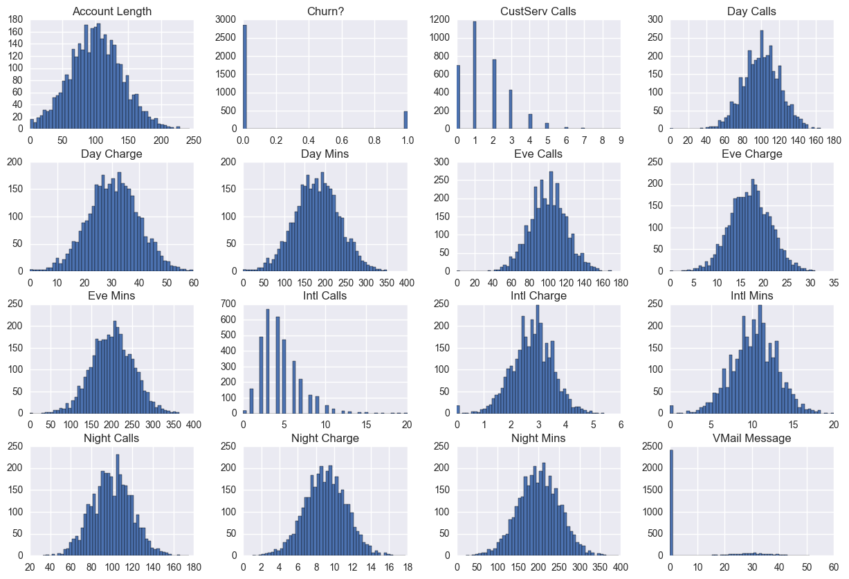
Exploring the distributions of the features, almost all of them following closely to normal distributions. The only exception being VMail message, with the majority of users having 0 VMail messages, likely because they have not subscribed to this service.

(df.groupby(['State','Churn?'])['Account Length'].count().unstack().sort_values(by=True, ascending = False)
.plot(kind='bar',stacked=True,figsize=(15, 5)))

<matplotlib.axes._subplots.AxesSubplot at 0x2085e7b8940>

png

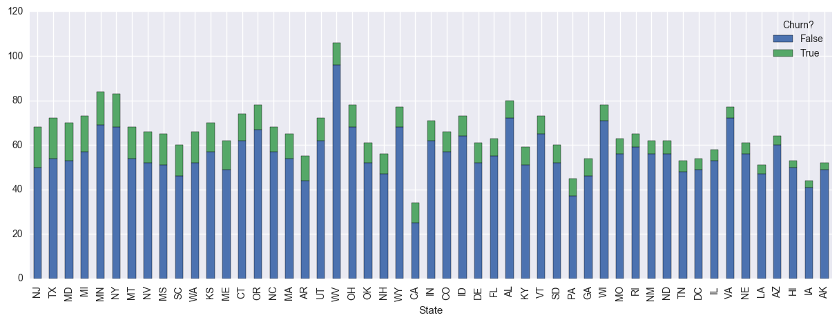
Exploring the churn-rate per state in the above visualization, we can see that there is a wide spread between churn-rate amoung different states, with NJ and TX having high churn and IA and AK with barely any. This islikely due to the different competetion markets across states, and should provide powerful discriminating features in a churn classifier.

sns.pairplot(df, hue="Churn?")

<seaborn.axisgrid.PairGrid at 0x208460a64a8>

png

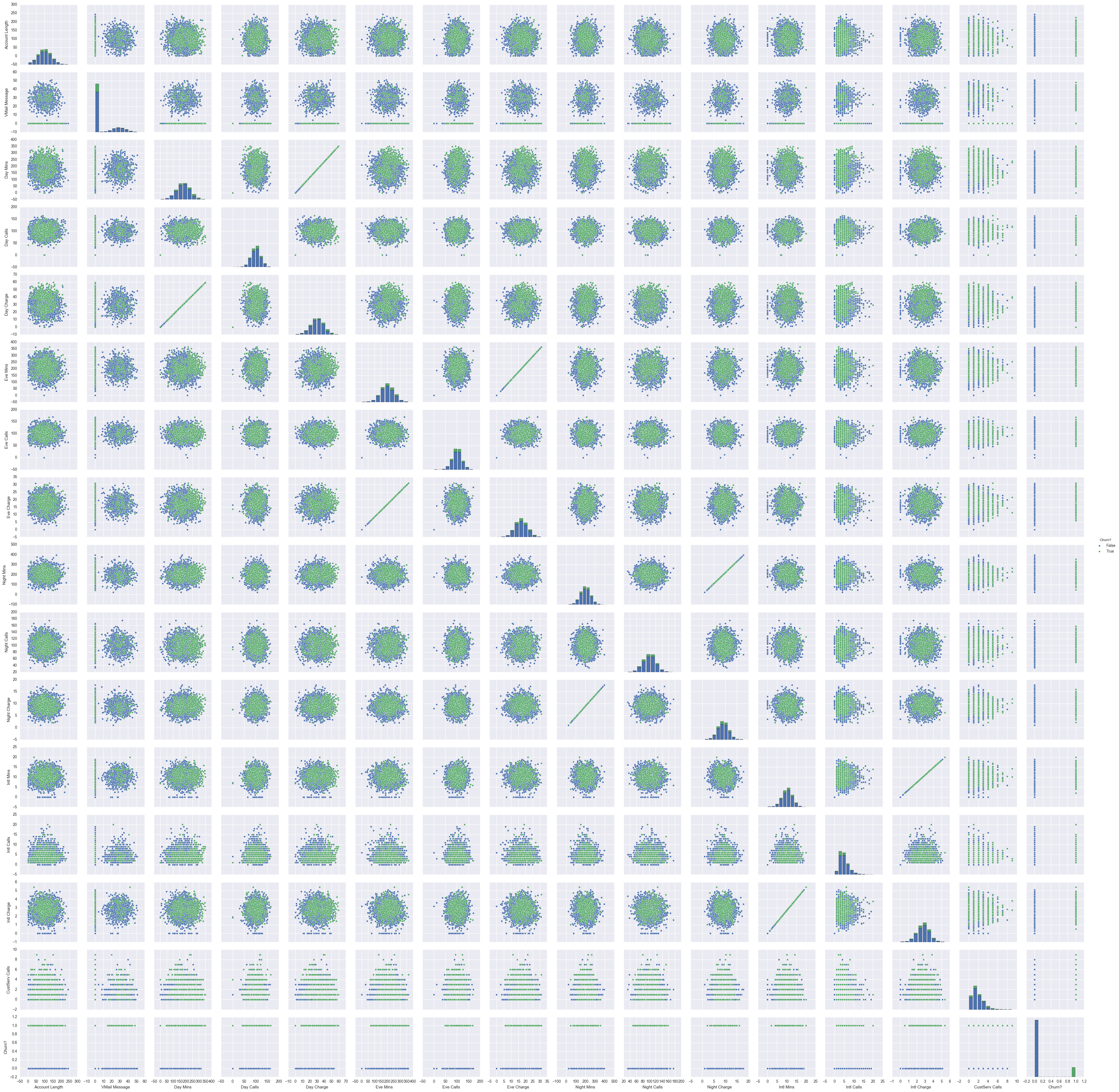
Reviewing the scatter matrix for each feature reveals the direct linear relationship between call minutes and their respective charges. These redundant features are removed from the dataset to prevent the potential negative influence of dependent features on the classifier. Although some features show a little seperating between churn labels, an obvious feature combination does not appear for discriminating churn customers. A higher dimensional classifier with further combinations of the features will required to build an adequate classifier.

filtered_features = ['Day Mins', 'Eve Mins', 'Night Mins', 'Intl Mins']
df = df.drop(filtered_features,1)
df.head()

	State	Account Length	Int'l Plan	VMail Plan	VMail Message	Day Calls	Day Charge	Eve Calls	Eve Charge	Night Calls	Night Charge	Intl Calls	Intl Charge	CustServ Calls	Churn?
0	KS	128	no	yes	25	110	45.07	99	16.78	91	11.01	3	2.70	1	False
1	OH	107	no	yes	26	123	27.47	103	16.62	103	11.45	3	3.70	1	False
2	NJ	137	no	no	0	114	41.38	110	10.30	104	7.32	5	3.29	0	False
3	OH	84	yes	no	0	71	50.90	88	5.26	89	8.86	7	1.78	2	False
4	OK	75	yes	no	0	113	28.34	122	12.61	121	8.41	3	2.73	3	False

mapping = {'yes': 1, 'no': 0}
df = df.replace({"Int'l Plan": mapping, 'VMail Plan': mapping})

#One Hot Encode States for classifer
state_df = df['State'].str.get_dummies() 
df = df.drop(['State'],1)
df = pd.concat([df,state_df],axis=1)

cols = ['Account Length', "Int'l Plan", 'VMail Plan', 'VMail Message',
       'Day Calls', 'Day Charge', 'Eve Calls', 'Eve Charge', 'Night Calls',
       'Night Charge', 'Intl Calls', 'Intl Charge', 'CustServ Calls',
       'AK', 'AL', 'AR', 'AZ', 'CA', 'CO', 'CT', 'DC', 'DE', 'FL', 'GA', 'HI',
       'IA', 'ID', 'IL', 'IN', 'KS', 'KY', 'LA', 'MA', 'MD', 'ME', 'MI', 'MN',
       'MO', 'MS', 'MT', 'NC', 'ND', 'NE', 'NH', 'NJ', 'NM', 'NV', 'NY', 'OH',
       'OK', 'OR', 'PA', 'RI', 'SC', 'SD', 'TN', 'TX', 'UT', 'VA', 'VT', 'WA',
       'WI', 'WV', 'WY','Churn?']
df = df[cols]
df.columns

Index(['Account Length', 'Int'l Plan', 'VMail Plan', 'VMail Message',
       'Day Calls', 'Day Charge', 'Eve Calls', 'Eve Charge', 'Night Calls',
       'Night Charge', 'Intl Calls', 'Intl Charge', 'CustServ Calls', 'AK',
       'AL', 'AR', 'AZ', 'CA', 'CO', 'CT', 'DC', 'DE', 'FL', 'GA', 'HI', 'IA',
       'ID', 'IL', 'IN', 'KS', 'KY', 'LA', 'MA', 'MD', 'ME', 'MI', 'MN', 'MO',
       'MS', 'MT', 'NC', 'ND', 'NE', 'NH', 'NJ', 'NM', 'NV', 'NY', 'OH', 'OK',
       'OR', 'PA', 'RI', 'SC', 'SD', 'TN', 'TX', 'UT', 'VA', 'VT', 'WA', 'WI',
       'WV', 'WY', 'Churn?'],
      dtype='object')

Model Development

Transforming the cleaned dataset into training and testing datasets, we can build the classifier by tuning the feature selector and estimator count with grid search. The weights are also redistributed to take into account the imbalance in the dataset.

train, test = train_test_split(df, test_size = 0.2)
X_train = train.as_matrix()[:,0:len(train.columns)-1]
y_train = train.as_matrix()[:,-1].astype(int)
y_train[y_train == True] = 1
y_train[y_train == False] = -1
X_test = test.as_matrix()[:,0:len(test.columns)-1]
y_test = test.as_matrix()[:,-1].astype(int)
y_test[y_test == True] = 1
y_test[y_test == False] = -1

feature_selector = SelectKBest(k=5)
weights = [2*1/len(y_train) if y_train[i] == 1 else 1/(2*len(y_train)) for i in range(len(y_train))]
weights = [wgt/sum(weights) for wgt in weights]
clf = IMLAdaBoostClassifier(n_estimators=10,weights=weights)
clf_pipe = Pipeline([('feature_selector', feature_selector), ('clf', clf)])
params = dict(feature_selector__k=[4,5,6,7,8],
              clf__n_estimators=[100,125,150,175,200])
iml_clf = GridSearchCV(clf_pipe, param_grid=params)

iml_clf.fit(X_train,y_train)
iml_clf.best_estimator_

Pipeline(steps=[('feature_selector', SelectKBest(k=5, score_func=<function f_classif at 0x000001B741D61BF8>)), ('clf', IMLAdaBoostClassifier(n_estimators=100,
           weights=[0.00026150627615061507, 0.00026150627615061507, 0.00026150627615061507, 0.00026150627615061507, 0.00026150627615061507, 0.00026150...3, 0.0010460251046024603, 0.00026150627615061507, 0.00026150627615061507, 0.00026150627615061507]))])

print ("score = " + str(iml_clf.score(X_test,y_test)))
preds = iml_clf.predict(X_test)
confusion_matrix(y_test,preds)

score = 0.842578710645





array([[483,  87],
       [ 18,  79]])

The resulting classifier takes the top 5 features and applies 100 weak learners to develop the final classifier, with a classification score of 84%. The classifier over predicts the number of churn clients, while under estimating the non-churning clients. This is the desired result of the classifier, with the specification stating we are more concerned with identifying potential churn clients over predicting non-churning ones.

feature_selector = SelectKBest(k=5)
clf = AdaBoostClassifier()
clf_pipe = Pipeline([('feature_selector', feature_selector), ('clf', clf)])
params = dict(feature_selector__k=[4,5,6,7,8],
              clf__n_estimators=[100,125,150,175,200])
skl_clf = GridSearchCV(clf_pipe, param_grid=params)

skl_clf.fit(X_train,y_train)
skl_clf.best_estimator_

Pipeline(steps=[('feature_selector', SelectKBest(k=8, score_func=<function f_classif at 0x000001B741D61BF8>)), ('clf', AdaBoostClassifier(algorithm='SAMME.R', base_estimator=None,
          learning_rate=1.0, n_estimators=100, random_state=None))])

print ("score = " + str(skl_clf.score(X_test,y_test)))
preds = skl_clf.predict(X_test)
confusion_matrix(y_test,preds)

score = 0.871064467766





array([[549,  21],
       [ 65,  32]])

When compared to the sklearn implementation of adaboost, the classifiers have similiar performance, with sklearn's classifier having 3% more classifcation accuracy. This gives confidence to the ability of our custom classifier to adequality classify real problems, but also indicates the existance of improvements we can embed into our classifier.

iml_features = iml_clf.best_estimator_.named_steps['feature_selector'].scores_

iml_top_features = sorted(range(len(iml_features)), key=lambda i: iml_features[i],reverse=True)[0:10]

df.columns[iml_top_features]

Index(['Int'l Plan', 'CustServ Calls', 'Day Charge', 'VMail Plan',
       'Eve Charge', 'VMail Message', 'Intl Charge', 'TX', 'Intl Calls', 'MS'],
      dtype='object')

Reviewing the feature importance scores, we can see that the plan usage and calls to the service center are important features, along with a couple of states that show high rates of churn. This information could be used to target these specific attributes for improvement in the telcomunication product.

Investment Plan

With the developed classifier, we can use its prediction power to develop an investment decision planner for deciding whether to invest into retention plans for certain customers. The following script provides the tools to transform new customer data to be fed into the investment decider, which takes the cost of retention, expected return on retained customers and the probability of customer churn from the developed classifier, and returns the expect monetary return from the individual retention investment. If the return is positive, an investment to retain the customer is recommended.

def data_transforms(df):
    filtered_features = ['Phone','Area Code','Day Mins', 'Eve Mins', 'Night Mins', 'Intl Mins']
    df = df.drop(filtered_features,1)
    mapping = {'yes': 1, 'no': 0}
    df = df.replace({"Int'l Plan": mapping, 'VMail Plan': mapping})
    state_df = df['State'].str.get_dummies()
    df = df.drop(['State'],1)
    df = pd.concat([df,state_df],axis=1)
    cols = ['Account Length', "Int'l Plan", 'VMail Plan', 'VMail Message',
       'Day Calls', 'Day Charge', 'Eve Calls', 'Eve Charge', 'Night Calls',
       'Night Charge', 'Intl Calls', 'Intl Charge', 'CustServ Calls',
       'AK', 'AL', 'AR', 'AZ', 'CA', 'CO', 'CT', 'DC', 'DE', 'FL', 'GA', 'HI',
       'IA', 'ID', 'IL', 'IN', 'KS', 'KY', 'LA', 'MA', 'MD', 'ME', 'MI', 'MN',
       'MO', 'MS', 'MT', 'NC', 'ND', 'NE', 'NH', 'NJ', 'NM', 'NV', 'NY', 'OH',
       'OK', 'OR', 'PA', 'RI', 'SC', 'SD', 'TN', 'TX', 'UT', 'VA', 'VT', 'WA',
       'WI', 'WV', 'WY']
    for cl in cols:
        if cl not in df.keys():
            df[cl] = 0
    df = df[cols]
    return df

def investment_decision(cost,roi,customer_data):
    inv_dec = []
    churn_prob = iml_clf.decision_function(customer_data)  
    for exp_churn in churn_prob:
        if exp_churn < 0:
            expected_return = -cost
        else:
            expected_return = (roi*exp_churn-cost)
        inv_dec.append(expected_return)
    return inv_dec

df = pd.read_csv("new_customers.csv")
df = data_transforms(df)
rslt = investment_decision(50,250,df)
for i,cust in enumerate(rslt):
    if cust > 0:
        print("Invest in retain customer " + str(i))

Invest in retain customer 15
Invest in retain customer 198
Invest in retain customer 542
Invest in retain customer 546
Invest in retain customer 694
Invest in retain customer 974
Invest in retain customer 978
Invest in retain customer 985
Invest in retain customer 1192
Invest in retain customer 1407
Invest in retain customer 1472
Invest in retain customer 1610
Invest in retain customer 2076
Invest in retain customer 2614
Invest in retain customer 2660
Invest in retain customer 2732
Invest in retain customer 2786
Invest in retain customer 2942
Invest in retain customer 3322

Future Work

Through comparing our classifier with those implemented in sklearn, it's clear that some optimization exist for improvement, the most obvious being added intelligence in the decision stub thresholding and weak learner development. Other work will include the validation of our investment planner and its success at different levels of investment cost and expected customer returns.

Bibliography

https://classroom.udacity.com/courses/ud675/lessons/367378584/concepts/3675485950923#
http://scikit-learn.org/stable/documentation.html
http://pandas.pydata.org/pandas-docs/stable/
http://seaborn.pydata.org/